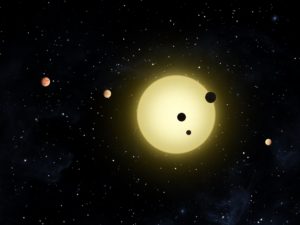
 In 1995 two astronomers, Michael Mayor and Didier Queloz, detected around the star 51 Pegasi the first extrasolar planet, 51 Pegasi b. This is a giant gaseous planet, with dimensions similar to Jupiter, orbiting around a Sun-like star. Sofar, almost 4000 extrasolar planet have been discovered, and their number is costantly increasing. The refinement of observational methods and the development of space missions make the search for exoplanets – in particular of those which might have suitable conditions for hosting forms of life – one of the most exciting topics of astronomy. Most extrasolar planest we know nowadays were discovered through the method of transits. Each time a planet is placed in the same direction of view as the observer, and passes in front of its star, it causes a periodic decrease, equal to the intensity of the brightness of the latter. Thanks to this effect, through ground or space telescopes, a periodic variation of the star’s brightness can be detected, whose periodicity is equal to the rotation period of the exoplanet. If we project the recorded variation of the star’s brightness on a chart, you will see regular dips in the points in which the planet passes in front of the star, obscuring a part of its disk. By studying the frequency of the curve of light, the astronomers obtain information on the period of revoluiion of the planet. Thanks to this method, we can detect both the orbital period and the dimension of the planet. In particular, since the obscured fraction of the star’s disk is proportional to the planet’s area, the decrease in percent brightness is a function both of the planet’s dimension, and of the host star. By indicating the brightness variation with ΔL, and with Rp and Rs the rays of the planet and of the star, we obtain that the percent variation of the brightness flow is given by:
ΔL/L = Rp2 / Rs2
From the brightness variation (therefore from the analysis of the curve of light recorded by the telescope), together with the star’s dimensions (usually estimated thanks to the models of nuclear physics), the astronomers can evaluate the dimensions of the planet.
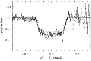
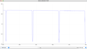
Curve of light of HD209458 b, the first planet discovered through the method of transits. The curves of light are not constituted by straight segments; first of all, in and out of transit is not instantaneous: it takes time for the planet to get in and completely out of the star disc. Moreover, there is also a period in which the planet is completely in front of the star’s surface, following a curve. This effect is due to the limb darkening, a physical phenomenon in which the host star’s brightness is not uniform over the entire surface, but is brighter in the middle of the line of sight, and weaker at the extremes of vision. Astronomers can create a statistical model in order to estimate the trend of limb darkening on the basis of photometric data, and of other information on the star (metallicity, equivalent temperature, gravity, …). Necessary material In order to realize our model of planetary system, and detector, we need the following materials:
- 2 Arduino cards;
- a stepper motor (motor) with a guidance module;
- a SD card reader for Arduino;
- a micro-SD to store data;
- three potentiometers;
- a photoresistance;
- a push button;
- two mini-breadboarda;
- straws;
- pins;
- a cardboard box;
- connection cables;
- toothpick;
- foil or plasticine.
First of all, let us realize the model of the planetary system. Take a straw and cut a piece of about 8 – 10 cm, straddling the folding part (about 3 cm before the folding part, and the rest after it). Fold the straw, and, through a pin, make a hole in the longer part. This will be the position in which you insert the planet. In order the keep the straw upright beyond the fold, we can place a small iron wire inside the straw, as an inner skeleton. In order to realize the planet, you can take the foil and roll it up in a tiny little ball with a 1-cm diametre, insert it in the toothpick, and place the whole thing on the straw. Inser the free end of the straw on the stepper motor, as shown in the following picture. 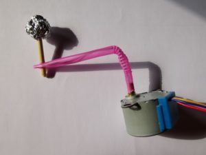 At this point, connect, through the special cables, the stepper motor to its guidance module. The stepper motor is an electric synchronous motor in direct current, which allows the subdivision of the rotation in small angles, or steps. In order to complete a full circle, 200 impulses are required. A stepper motor is very precise, quick, and easy to control through an electronic card, called driver, which is the true protagonist of the control of the stepper motor. The rotation speeed depends from the waiting time between one impulse and the other inside the single rotation cycles. In order to modify the rotation speed of the planetary system, we will use a potentiometer, whereas to change the direction of rotation we will use a button. In order to connect all the components, you can follow this scheme:
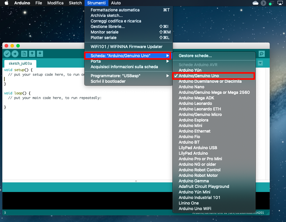
 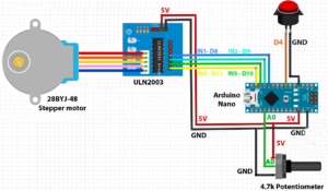 After arranging all connections, you can upload the code on the Arduino card in order to make the planet rotate. First of all, connect, with a suitable cable, the Arduino card to your computer, where you have previously installed the software to control and program the Arduino card. After opening the Arduino IDE, go to tools/card and select Arduino/Genuino Uno, then go to tools/port and select the port to which Arduino is connected. In this way, we set the work environment of Arduino, and we can starr to write the code for the planeta The code can be downloaded here.
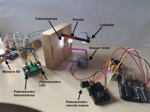
After arranging all connections, you can upload the code on the Arduino card in order to make the planet rotate. First of all, connect, with a suitable cable, the Arduino card to your computer, where you have previously installed the software to control and program the Arduino card. After opening the Arduino IDE, go to tools/card and select Arduino/Genuino Uno, then go to tools/port and select the port to which Arduino is connected. In this way, we set the work environment of Arduino, and we can starr to write the code for the planeta The code can be downloaded here: 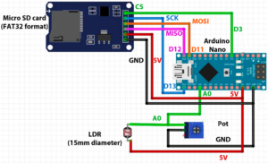 At this point, we can connect this second Arduino card to the computer too, and upload the new code. First of all, let us connect, with its appropriate cable, the Arduino card to the computer. After opening the Arduino IDE, we can go to tools/card and select Arduino/Genuino Uno and then go to tools/port and select the port to which Arduino is connected. In this way, we set the working environment of Arduino, and we can start writing the code for the sensor. The code can be downloaded here. The peculiarity of this code is that in the void loop there is a series of instructions which enable to store in the memory card the values of brightness in function of time. In particular, the datalogger operator allows you to open the SD card and write a file with a txt extension. Once you have created the data.txt file, the software records the data on the SD card, following the formatting we have decided. In this case, the data.txt file will report in each line the value of the light intensity recorded by the photoresistance, with a decimal digit, and the instant of time in milliseconds, always with a decimal digit. Finally, through Arduino’s serial plotter, we can see in real time the curve of light. In order to get access to the serial plotter, you can simply go to tools/serial plotter. As the “planet” passes in front of the “star”, the value of brightness decreases, down to a minimum value. In this phase, the planet is completely in front of the star and totally obscures its light. Finally, when the planet starts to exit the star disk, the star’s brightness rincreases again, until it reaches the initial values. The light of the star remains in its maximum value, until the planet ha completed its orbits, reducing once again the light of the star. The image below shows the star-planet-detector system we described above, with an example of light curve. Here you can see an example of the data.txt file.
 At this point, all we have to do is varying a few parameters – as for example the rotation speed, the dimensions of the planet, the distance of the planet from the star – and see how the relative curves of ligh change. You can learn more about the method of transits with a simulation realized with Scratch.

